▷ 前を見る
11.2 等値面(isosurface)
等値面(isosurface)は、設定した関数の計算値が同じ値になる点を抽出し面を生成する機能である。まなざまな組み込み関数などを組み合わせること多彩な面を生成できる。
< isosurface の構文 >
|
isosurface {
function { FUNCTION_ITEMS }
[ contained_by { SPHERE | BOX } ]
[ threshold FLOAT_VALUE ]
[ accuracy FLOAT_VALUE ]
[ max_gradient FLOAT_VALUE ]
[ evaluate P0, P1, P2 ]
[ open ]
[ max_trace INTEGER ] | [ all_intersections ]
[ OBJECT_MODIFIERS... ]
}
|
| isosurface |
等値面のキーワード |
| function { FUNCTION_ITEMS } |
等値面を生成する関数の設定 ▷「11.2-5 関数」 |
| contained_by { SPHERE | BOX } |
等値面を生成する範囲の設定、球またはボックスを使用 [ディフォルト:box{-1,1} ] ▷「11.2-1 生成範囲」 |
| threshold FLOAT_VALUE |
等値面を生成する値(閾値)設定、関数の計算値がこの値になる点から面を生成する。[ディフォルト:0] ▷「11.2-2 閾値」 |
| accuracy FLOAT_VALUE |
再帰分割の値の設定、小さいほど正確な値が得られる。[ディフォルト:0.001] |
| max_gradient FLOAT_VALUE |
関数の最大勾配の設定 [ディフォルト:1.1] ▷「11.2-3 最大勾配関数」 |
| evaluate P0, P1, P2 |
最大勾配を動的に探索する機能。P0は最小値、P1は最大値、P2は減衰値で設定する。 |
| open |
contained_byで設定された物体の形状部分を生成しない設定、立体ではなく等値面のみの生成となる。▷「11.2-4 オープン」 |
| max_trace INTEGER |
CSGにおける交差面のチェック回数の設定 |
| all_intersections |
CSGにおける交差面を全てチェックする。 |
| OBJECT_MODIFIERS... |
物体の変形・テクスチャなどの設定 |
11.2-1 生成範囲(contained_by)
contained_by で面の生成範囲を設定する。生成範囲は、ボックスまたは球で範囲設定を行う。図11.2-1は、生成範囲であるボックスの中に等値面である円錐が生成されている。この図ではわかり易いようにボックスを半透明で描いている。
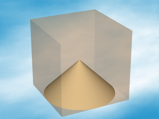 |
| 図11.2-1 生成範囲ボックスと等値面 |
//--------------- Fig. 11.2-1 contained_by
#version 3.7
#include "colors.inc"
global_settings
{assumed_gamma 2.2}
camera{
location<10,20,10>
sky<0,0,1>
right <-image_width/image_height,0,0>
look_at<0,0,0>
angle 20
}
light_source {<300,500,500> color 2
parallel point_at <0,0,0>}
//=============================== /// isosurface ///
isosurface {
function { sqrt(pow(x,2) + pow(y,2)) + z }
contained_by { box { -2, 2 } } // <<<--- contained_by
max_gradient 1.8
pigment{color rgb<1,0.88,0.65>}
}
box { -2, 2 pigment{color rgbt<0.8,0.6,0.4,0.7>} }
//----------------sky
sky_sphere{
pigment{
wrinkles
color_map{
[ 0.4 SkyBlue]
[ 0.9 White ]
}
scale <1, 0.2, 0.2>
}
}
11.2-2 閾値(threshold)
閾値(threshold)は等値面の値である。設定した関数の計算値が、閾値に等しくなる点の集合から面が生成される。次式は、半径が2の球の式である。
sqrt(pow(x,2) + pow(y,2) + pow(z,2)) = 2
等値面の記述は、閾値(threshold)を用いると次のようになる。これで半径2の球体が生成される。
isosurface {
function { sqrt(pow(x,2) + pow(y,2) + pow(z,2)) }
contained_by { box { -2, 2 } }
threshold 2
}
または、次の記述でも同じである。(threshold のデフォルトは 0 なので記述省略)
isosurface {
function { sqrt(pow(x,2) + pow(y,2) + pow(z,2)) - 2 }
contained_by { box { -2, 2 } }
}
11.2-3 最大勾配(max_gradient)
関数の最大勾配の設定をする。値が低すぎると、割れ目ができたり穴が開いたりするが、高すぎると計算が遅くなる。必要に応じて値を調整する必要がある。図11.2-3の左側の等値面は max_gradient を 3 としたもので、右側の等値面は max_gradient 記述を省略しディフォルトの 1.1 が使われ、この値ではうまく等値面が生成できていない。
 |
| 図11.2-3 最大勾配の値による比較 |
//--------------- Fig. 11.2-3 max_gradient
#version 3.7
#include "colors.inc"
global_settings
{assumed_gamma 2.2}
camera{
location<10,20,10>
sky<0,0,1>
right <-image_width/image_height,0,0>
look_at<0,0,0>
angle 20
}
light_source {<300,500,500> color 2
parallel point_at <0,0,0>}
//=================== /// isosurface (a) ///
isosurface {
function { pow(x,2) + z-0.5 }
contained_by { box { -2, 2 } }
max_gradient 3 // <<<--------max_gradient
pigment{color rgb<1,0.88,0.65>}
translate <2,0,1>
}
//=================== /// isosurface (b) ///
isosurface {
function { pow(x,2) + z-0.5 }
contained_by { box { -2, 2 } }
//max_gradient 3
pigment{color rgb<1,0.88,0.65>}
translate <-2,0,1>
}
//----------------sky
sky_sphere{
pigment{
wrinkles
color_map{
[ 0.4 SkyBlue]
[ 0.9 White ]
}
scale <1, 0.2, 0.2>
}
}
11.2-4 オープン(open)
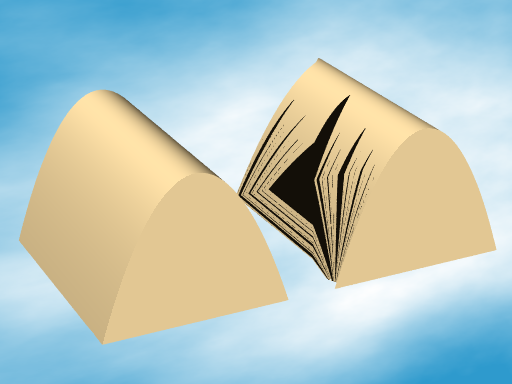
等値面は、contained_by で設定された形状(ボックスまたは球)の内側で生成される。等値面と生成範囲の立体が交差するとき、その交差面もディフォルトで生成される。open はこのような面を生成しない設定である。図11,2-4は、open を設定した2つの等値面を表している。
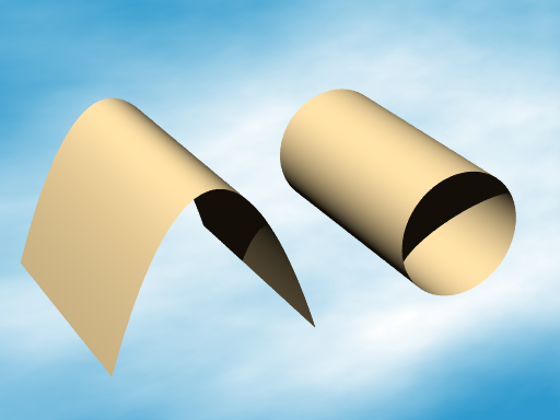 |
| 図11.2-4 オープンを設定した等値面 |
//--------------- Fig. 11.2-4 open
#version 3.7
#include "colors.inc"
global_settings
{assumed_gamma 2.2}
camera{
location<10,20,10>
sky<0,0,1>
right <-image_width/image_height,0,0>
look_at<0,0,0>
angle 20
}
light_source {<300,500,500> color 2
parallel point_at <0,0,0>}
//======================== /// isosurface (a) ///
isosurface {
function { pow(x,2) + z-0.5 }
contained_by { box { -2, 2 } }
max_gradient 3
open // <<<-----------------open
pigment{color rgb<1,0.88,0.65>}
translate <2,0,1>
}
//======================== /// isosurface (b) ///
isosurface {
function { sqrt(pow(x,2) + pow(z,2)) - 1 }
contained_by { box { -2, 2 } }
max_gradient 3
open // <<<-----------------open
pigment{color rgb<1,0.88,0.65>}
translate <-2,0,0>
}
//----------------sky
sky_sphere{
pigment{
wrinkles
color_map{
[ 0.4 SkyBlue]
[ 0.9 White ]
}
scale <1, 0.2, 0.2>
}
}
11.2-5 関数(function)
関数の作り方しだいで、単純な形状から複雑なものまでさまざまな3次元面を作成できる。functions.inc に定義されいる関数も使うことができる。4つの例を示す。
(a) 平面式による等値面
図11.2-5a は、次の関数を使っている。
関数 x + y + z = 0
この関数の値を満たす等値面を生成している。contained_by で立方体のボックスを設定しているので、等値面の端部がボックスでカットされている。
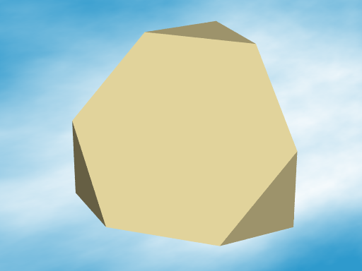 |
| 図11.2-5a 平面式による等値面 |
//--------------- Fig. 11.2-5a function
#version 3.7
#include "colors.inc"
#include "Woods.inc"
#include "stones.inc"
global_settings
{assumed_gamma 2.2}
camera{
location<10,20,10>
sky<0,0,1>
right <-image_width/image_height,0,0>
look_at<0,0,0>
angle 20
}
light_source {<300,500,500> color 1.7
parallel point_at <0,0,0>}
//====================== 5a /// isosurface ///
isosurface {
function { x + y + z } // <<<--------function (a)
contained_by { box { -2, 2 } }
max_gradient 1.8
pigment{color rgb<0.8,0.75,0.55>}
}
//----------------sky
sky_sphere{
pigment{
wrinkles
color_map{
[ 0.4 SkyBlue]
[ 0.9 White ]
}
scale <1, 0.2, 0.2>
}
}
(b) ノイズ関数による等値面 1
POV-Ray が内部関数として持っているノイズ関数を使った例である。ボーゾ(bozo)パターンのようなノイズを作り出す。この関数は 0~1 の数値を返すので、ここでは 0.5 の値の等値面を指定したことになる。
関数 f_noise3d(x, y, z) - 0.5 = 0
この例でも、contained_by で立方体のボックスを設定しているので、等値面がそれに沿ってカットされた形状が生成されている。
 |
| 図11.2-5b ノイズ関数による等値面1 |
//--------------- Fig. 11.2-5b function
#version 3.7
#include "colors.inc"
#include "Woods.inc"
#include "stones.inc"
#include "shapes.inc"
global_settings
{assumed_gamma 2.2}
camera{
location<10,20,10>
sky<0,0,1>
right <-image_width/image_height,0,0>
look_at<0,0,0>
angle 20
}
light_source {<300,500,500> color 1.7
parallel point_at <0,0,0>}
//======================= 5b /// isosurface ///
isosurface {
function { f_noise3d(x, y, z) - 0.5 } // <<<--function (b)
contained_by { box { -2, 2 } }
max_gradient 1.8
pigment{color rgb<0.8,0.75,0.55>}
}
//----------------sky
sky_sphere{
pigment{
wrinkles
color_map{
[ 0.4 SkyBlue]
[ 0.9 White ]
}
scale <1, 0.2, 0.2>
}
}
(c) ノイズ関数による等値面 2
関数は (1) と同じノイズ関数で、z を 0 として、これに z を加えている。その効果としては、ハイトフィールドのような物体になるのが特徴である。
関数 z + f_noise3d(x, y, 0) = 0
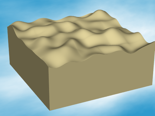 |
| 図11.2-5c ノイズ関数による等値面 2 |
//--------------- Fig. 11.2-5c function
#version 3.7
#include "colors.inc"
#include "Woods.inc"
#include "stones.inc"
#include "shapes.inc"
global_settings
{assumed_gamma 2.2}
camera{
location<10,20,10>
sky<0,0,1>
right <-image_width/image_height,0,0>
look_at<0,0,0>
angle 20
}
light_source {<300,500,500> color 1.7
parallel point_at <0,0,0>}
//======================== 5c /// isosurface ///
isosurface {
function { z+f_noise3d(x, y, 0) } // <<<--function (c)
contained_by { box { -3,3 } }
max_gradient 1.8
pigment{color rgb<0.8,0.75,0.55>}
translate z*2
}
//----------------sky
sky_sphere{
pigment{
wrinkles
color_map{
[ 0.4 SkyBlue]
[ 0.9 White ]
}
scale <1, 0.2, 0.2>
}
}
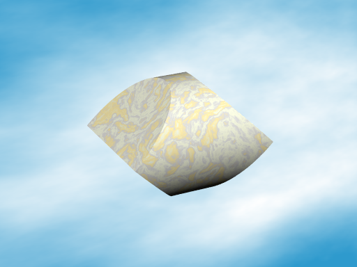
(d) ノイズ関数による等値面 3
次の関数は、ノイズ関数を球面に適用している例である。 (1) と同じ関数により球面上の不規則な凹凸を表現している。ノイズ関数へ乗算がノイズ強度の調節、x,y,z のパラメータに対する乗算がスケール調節になっている。
関数 f_sphere(x, y, z, 1.6) - f_noise3d(x*5, y*5, z*5) * 0.5 = 0
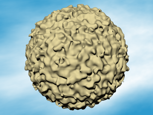 |
| 図11.2-5d ノイズ関数による等値面 3 |
//--------------- Fig. 11.2-5d function
#version 3.7
#include "colors.inc"
#include "Woods.inc"
#include "stones.inc"
#include "shapes.inc"
global_settings
{assumed_gamma 2.2}
camera{
location<10,20,10>
sky<0,0,1>
right <-image_width/image_height,0,0>
look_at<0,0,0>
angle 20
}
light_source {<300,500,500> color 1.7
parallel point_at <0,0,0>}
//======================== 5d /// isosurface ///
isosurface {
function { f_sphere(x, y, z, 1.6)
-f_noise3d(x*5, y*5, z*5)*0.5 } // <<<--function (d)
contained_by { box { -2, 2 } }
max_gradient 3
scale 1.5
pigment{color rgb<0.8,0.75,0.55>}
}
//----------------sky
sky_sphere{
pigment{
wrinkles
color_map{
[ 0.4 SkyBlue]
[ 0.9 White ]
}
scale <1, 0.2, 0.2>
}
}
11.2-6 関数の応用
min 関数、max 関数の利用で、関数の論理演算が可能になる。これにより CSG と同じように物体の論理和、論理積、論理差による物体を生成できる。関数から関数への遷移を記述するとブロブ機能も実現できる。
▷「11.3 CSG」参照
(a) 論理和: min 関数の利用
2つの関数を次の例に示すように、 min 関数を使って記述すると、論理和(union)を生成することができる。下記例は POV-Ray の記述例であり、FNA、FNB は定義された任意の関数を意味する。 ▷「11.3-1 論理和」参照
#declare FNA=function{sqrt(pow(y,2)+pow(z,2))-0.8}
#declare FNB=function{abs(x)+abs(z)-1}
isosurface {
function { min( FNA(x,y,z), FNB(x,y,z) ) } // union
contained_by { box { -2, 2 } }
max_gradient 1.8
}
 |
| 図11.2-6a 関数の論理和 |
//--------------- Fig. 11.2-6a CSG (union)
#version 3.7
#include "colors.inc"
#include "Woods.inc"
#include "stones.inc"
global_settings
{assumed_gamma 2.2}
camera{
location<10,20,10>
sky<0,0,1>
right <-image_width/image_height,0,0>
look_at<0,0,0>
angle 20
}
light_source {<300,500,500> color 1.7
parallel point_at <0,0,0>}
//======================== 6a CSG /// isosurface ///
#declare FNA=function{sqrt(pow(y,2)+pow(z,2))-0.8}
#declare FNB=function{abs(x)+abs(z)-1}
isosurface {
function { min( FNA(x,y,z), FNB(x,y,z) ) } // <<<--union
contained_by { box { -2, 2 } }
max_gradient 1.8
texture {T_Grnt1}
scale 1.8
}
//----------------sky
sky_sphere{
pigment{
wrinkles
color_map{
[ 0.4 SkyBlue]
[ 0.9 White ]
}
scale <1, 0.2, 0.2>
}
}
(b) 論理積: max 関数の利用
2つの関数を次の例の示にすように、 max 関数を使って記述すると、論理積(intersection)の生成ができる。下記例は 上記と同様に、FNA、FNB は定義された任意の関数を意味する。 ▷「11.3-2 論理積」参照
#declare FNA=function{sqrt(pow(y,2)+pow(z,2))-0.8}
#declare FNB=function{abs(x)+abs(z)-1}
isosurface {
function { max( FNA(x,y,z), FNB(x,y,z) ) } // intersection
contained_by { box { -2, 2 } }
max_gradient 1.8
}
 |
| 図11.2-6b 関数の論理積 |
//--------------- Fig. 11.2-6b CSG (intersection)
#version 3.7
#include "colors.inc"
#include "Woods.inc"
#include "stones.inc"
global_settings
{assumed_gamma 2.2}
camera{
location<10,20,10>
sky<0,0,1>
right <-image_width/image_height,0,0>
look_at<0,0,0>
angle 20
}
light_source {<300,500,500> color 1.7
parallel point_at <0,0,0>}
//======================== 6b CSG /// isosurface ///
#declare FNA=function{sqrt(pow(y,2)+pow(z,2))-0.8}
#declare FNB=function{abs(x)+abs(z)-1}
isosurface {
function { max( FNA(x,y,z), FNB(x,y,z) ) } // <<<--intersection
contained_by { box { -2, 2 } }
max_gradient 1.8
texture {T_Grnt1}
scale 1.8
}
//----------------sky
sky_sphere{
pigment{
wrinkles
color_map{
[ 0.4 SkyBlue]
[ 0.9 White ]
}
scale <1, 0.2, 0.2>
}
}
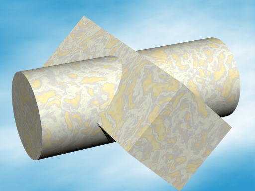
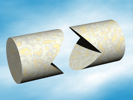
(c) 論理差: min 関数の利用、引く関数に - をつける。
2つの関数を次の例の示にすように、 max 関数を使って記述すると、論理差(difference)の生成ができる。削除したい共通部分があり、残さないでよい関数には - を付ける。下記例では、関数 FNB である。 ▷「11.3-3 論理差」参照
#declare FNA=function{sqrt(pow(y,2)+pow(z,2))-0.8}
#declare FNB=function{abs(x)+abs(z)-1}
isosurface {
function { max( FNA(x,y,z), -FNB(x,y,z) ) } // difference
contained_by { box { -2, 2 } }
max_gradient 1.8
}
 |
| 図11.2-6c 関数の論理差 |
//--------------- Fig. 11.2-6c CSG (difference)
#version 3.7
#include "colors.inc"
#include "Woods.inc"
#include "stones.inc"
global_settings
{assumed_gamma 2.2}
camera{
location<10,20,10>
sky<0,0,1>
right <-image_width/image_height,0,0>
look_at<0,0,0>
angle 20
}
light_source {<300,500,500> color 1.7
parallel point_at <0,0,0>}
//======================== 6c CSG /// isosurface ///
#declare FNA=function{sqrt(pow(y,2)+pow(z,2))-0.8}
#declare FNB=function{abs(x)+abs(z)-1}
isosurface {
function { max( FNA(x,y,z), -FNB(x,y,z) ) } // <<<--difference
contained_by { box { -2, 2 } }
max_gradient 1.8
texture {T_Grnt1}
scale 1.8
}
//----------------sky
sky_sphere{
pigment{
wrinkles
color_map{
[ 0.4 SkyBlue]
[ 0.9 White ]
}
scale <1, 0.2, 0.2>
}
}
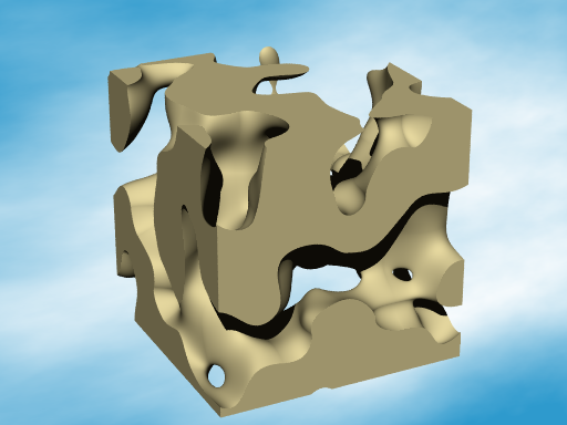
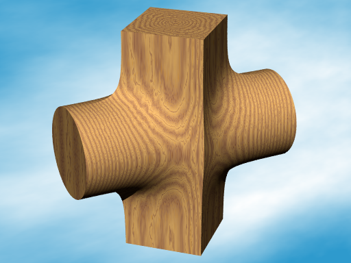
(d) ブロブ
関数から関数への遷移を記述すると、ブロブ(blob)の機能が実現できる。次の例の示にすように、 pow 関数を利用して記述している。Blob_threshold は遷移の滑らかさの程度を示し、値が小さいほどシャープになる。 ▷「11.1-19 ブロブ」参照
#declare FNA=function{sqrt(pow(y,2)+pow(z,2))-0.8}
#declare FNB=function{abs(x)+abs(y)-1}
#declare Blob_threshold=0.01;
isosurface {
function {
1+Blob_threshold
- pow( Blob_threshold, FNA(x,y,z) ) // blob FNA
- pow( Blob_threshold, FNB(x,y,z) ) // blob FNB
}
contained_by { box { -2, 2 } }
max_gradient 6
}
 |
| 図11.2-6d 関数のブロブ |
//--------------- Fig. 11.2-6d blob
#version 3.7
#include "colors.inc"
#include "Woods.inc"
#include "stones.inc"
global_settings
{assumed_gamma 2.2}
camera{
location<10,20,10>
sky<0,0,1>
right <-image_width/image_height,0,0>
look_at<0,0,0>
angle 20
}
light_source {<300,500,500> color 1.7
parallel point_at <0,0,0>}
//======================== 6d blob /// isosurface ///
#declare FNA=function{sqrt(pow(y,2)+pow(z,2))-0.8}
#declare FNB=function{abs(x)+abs(y)-1}
#declare Blob_threshold=0.01;
isosurface {
function { // <<<--- blob
1+Blob_threshold
- pow( Blob_threshold, FNA(x,y,z) )
- pow( Blob_threshold, FNB(x,y,z) )
}
contained_by { box { -2, 2 } }
max_gradient 6
texture {T_Wood7 scale 0.5}
scale 1.4
}
//----------------sky
sky_sphere{
pigment{
wrinkles
color_map{
[ 0.4 SkyBlue]
[ 0.9 White ]
}
scale <1, 0.2, 0.2>
}
}
▷ 次を見る